Sensor Fusion, Ultra Low Power Inference, and the architecture decisions that separate a model from a shipping product.
Every embedded ML project passes through the same sequence of uncomfortable decisions. The model trains fine on your laptop. It quantises to INT8 without catastrophic accuracy loss. Then someone asks you to run it on a Cortex-M33 that is simultaneously maintaining a BLE connection, reading three sensors at 200 Hz, and surviving on a 400 mAh battery for six months.
At that point, “edge AI” stops being a model problem and becomes a firmware architecture problem. The ten patterns below describe the decisions that separate a trained model from a certified, deployed wireless IoT product. They are ordered by the sequence in which they typically surface in a real project, not by difficulty or importance, because both vary by application. They apply whether you are building in-house or engaging an embedded systems development company for integration support.
Pattern 1: Inference trigger strategy: interrupt-driven, scheduled, or always-on
The first decision in any edge AI + wireless IoT hardware development project is: when does inference run?
Three strategies exist, and none is universally correct.
Interrupt-driven inference fires only when a hardware condition is met: a threshold crossing on an accelerometer, a GPIO signal from a photodetector, or a radio event flag. The interrupt wakes the CPU, runs inference, and the device returns to a low-power state. This approach minimises average current draw and is appropriate for anomaly detection (where the interesting event is rare) and gesture recognition (where the sensor delivers a clear trigger signal). The firmware risk is interrupt priority: if the inference callback occupies the CPU long enough to cause a BLE event to be missed, connection supervision will drop the link.
Scheduled inference runs at a fixed interval set by a hardware timer: every 100 ms, every 500 ms, every 10 s. This is predictable, easy to power-profile, and plays well with duty-cycled BLE advertising or connection intervals. It works for vital-sign monitoring (where the signal is continuous and periodic sampling makes sense) and environmental sensing. The trade-off is that inference fires even when the input signal is uninteresting, consuming energy on trivial classifications.
Always-on inference (sometimes called continuous inference) runs the model as fast as the hardware allows, relying on a dedicated always-on DSP or NPU core that draws significantly less power than the main application CPU. Nordic’s Axon NPU in the nRF54LM20B is designed for this mode: inference at 3.0 mA average current, with the Cortex-M33 asleep during inference execution. Ambiq’s SPOT technology enables the Cortex-M55 in the Apollo510B to run inference at clock frequencies that keep average power in the sub-1 mW range during sustained inference workloads.
Practical rule: use interrupt-driven for detection tasks, scheduled for monitoring tasks, and always-on only when a dedicated low-power inference core is available and the inference workload has been profiled on hardware.
Pattern 2: ML framework selection: TFLite Micro, NanoEdge AI Studio, or ONNX Runtime
The framework you choose determines your entire inference pipeline: the operators available, the quantisation format, the memory allocator, the microcontroller targets supported, and the toolchain your team needs to maintain.
[TFLite Micro (now LiteRT for Microcontrollers)]{.underline} is the most widely deployed embedded inference engine in 2026. It supports Cortex-M0 through M55, RISC-V, and Tensilica targets, with vendor-specific backends for Arm Ethos-U (Nordic Axon NPU, Alif Ensemble), NXP eIQ, and ST X-CUBE-AI. INT8 quantisation is well-supported. The kernel set is production-proven. The main trade-off is code size: a minimal TFLite Micro build is around 20–30 kB of flash before the model is added. Tooling for model conversion and debugging is mature.
NanoEdge AI Studio (STMicroelectronics, now free for STM32 targets) generates optimised C libraries directly from your sensor data, with no model design required. The Studio iterates across millions of algorithm candidates to find the smallest, most accurate library for your signal type and your target MCU. Generated libraries run down to Cortex-M0 with footprints under 10 kB. The trade-off is that you cannot customise the model architecture, and the output is an STM32-optimised static library, not portable C.
ONNX Runtime targets higher-performance MCUs and application processors (Cortex-M55+, i.MX RT, Cortex-A) and handles models exported from PyTorch or TensorFlow in the standard ONNX format. It is a better fit for vision and audio models that have outgrown the TFLite Micro operator set.
Framework selection quick reference:
| Framework | Minimum flash | Quantisation | Target MCU range | Best for |
|---|---|---|---|---|
| TFLite Micro / LiteRT | ~20 kB + model | INT8, INT4 | Cortex-M0 → M55 | Classification, anomaly, keyword |
| NanoEdge AI Studio | < 10 kB | Internal (STM32 only) | Cortex-M0 → M7 | Anomaly, classification from sensor data, no-code |
| ONNX Runtime | ~100 kB+ | FP32, INT8 | Cortex-M55+, A-class | Vision, audio, complex models |
Pattern 3: Flash and RAM partitioning: the constraint that drives every other decision
On a device running both an ML model and a wireless stack, the flash and RAM map is the earliest and most consequential firmware architecture decision. Get it wrong here and you will be refactoring the memory map six weeks into integration.
A practical example for a 1 MB / 256 kB device running BLE and TFLite Micro:
| Region | Flash allocation | RAM allocation |
|---|---|---|
| BLE Controller (e.g., Nordic SoftDevice) | 160 kB | 24 kB |
| RTOS + bootloader | 48 kB | 16 kB |
| TFLite Micro runtime | 28 kB | n/a |
| ML model weights (INT8) | 80–120 kB | n/a |
| Inference arena (activation tensors) | n/a | 48–96 kB |
| Application code | 200–250 kB | 32 kB |
| DFU slot (OTA) | ~200 kB | n/a |
| Remaining headroom | ~90–120 kB | ~48–88 kB |
The inference arena is the critical RAM allocation: TFLite Micro allocates a static tensor arena at startup and uses it for all activation tensors during inference. If the arena is too small, inference fails at runtime with a cryptic allocation error. If it is too large, you have evicted RAM that the RTOS scheduler or BLE stack would have used. Profiling the exact arena requirement for your model (using RecordingMicroAllocator or the Edge Impulse memory profiler) should happen before any RAM map is finalised.
Silicon Labs’ edge AI integration guide recommends separating the BLE network processor concerns from the application core at the architecture stage, even on single-core devices, by using a task/priority model that gives BLE ISRs higher priority than inference tasks.
Pattern 4: Model quantisation and compression: reaching the INT8 / INT4 target without accuracy loss
A float32 model that achieves 94% accuracy in your training notebook will consume 4× the flash of an INT8 equivalent. On a 256 kB flash device, float32 is usually not an option. INT8 post-training quantisation is the standard first step.
Post-training quantisation (PTQ) converts float32 weights to INT8 after training using a calibration dataset of 100–1000 representative inputs. On most classification and anomaly detection tasks for sensor data (accelerometer, temperature, audio), the accuracy drop is under 1–2%. For models with unusual weight distributions or heavy use of batch normalisation layers, PTQ can cause larger drops, in which case quantisation-aware training (QAT) inserts fake quantisation into the forward pass during training, typically recovering the lost accuracy at the cost of a longer training run.
INT4 quantisation (supported in LiteRT / TFLite Micro from mid-2025) halves the model weight footprint again, reaching under 30 kB for many production-grade classification models. The accuracy risk is higher and requires QAT, but for well-understood task types (keyword spotting, gesture classification, vibration anomaly) the results are now production-viable on the right target.
Knowledge distillation (training a small “student” model to mimic a larger “teacher”) is worth considering when the model task is complex but the accuracy of a directly-trained small model is insufficient. The student model can be INT8 quantised after distillation, combining the accuracy benefits of the larger model with the size benefits of the smaller architecture.
Rule of thumb: budget 50–100 kB of flash for a production-grade INT8 classification or anomaly model on a BLE + ML device, and profile the INT8 accuracy drop on your validation set before committing to hardware.
Pattern 5: Sensor fusion pipeline architecture: UWB, IMU, and LiDAR on a single device
Sensor fusion for wireless IoT is not simply averaging two sensor readings. It involves managing sampling rates, alignment timestamps, coordinate frame transformations, and the inference pipeline across sensors that may have different update rates, noise characteristics, and failure modes.
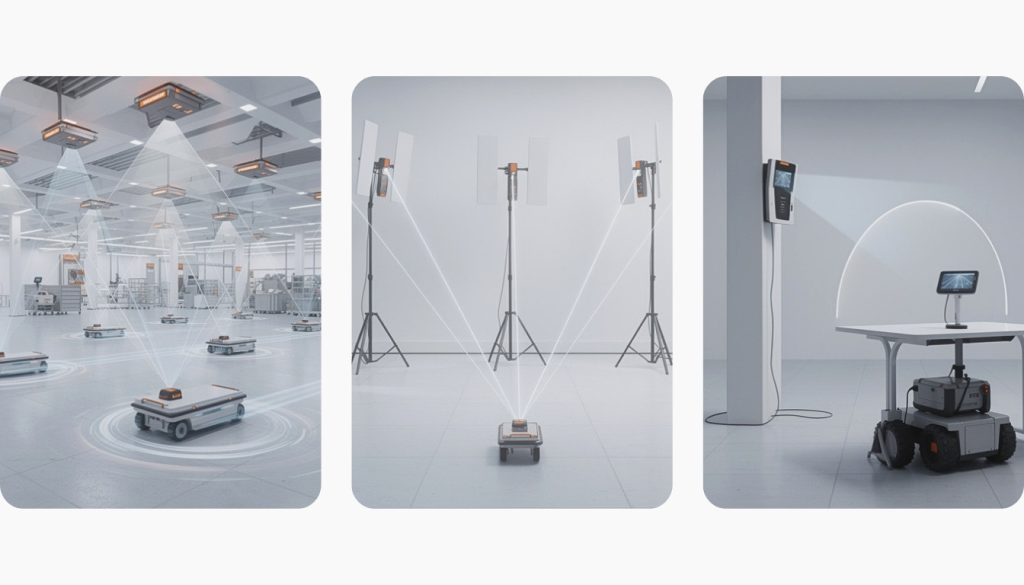
A typical UWB + IMU fusion pipeline for indoor robotics:
- UWB ranging produces a position estimate (X, Y, or X, Y, Z) at 10–50 Hz. Each ranging event requires a radio transaction, which competes with BLE advertising or connection events for the RF subsystem.
- IMU (accelerometer + gyroscope) produces acceleration and angular rate data at 100–400 Hz. A Kalman filter or complementary filter fuses the IMU output with the UWB position to produce a higher-rate, lower-latency state estimate that bridges the gaps between UWB ranging events.
- LiDAR (for ground robotics) produces a point cloud at 10–20 Hz. The point cloud data volume is large, too large to transmit over BLE without significant compression or subsampling. Local processing (occupancy grid, obstacle map update) must happen on-device before any wireless transmission.
The embedded AI component typically sits on top of this fusion stack: a classifier that takes the fused state vector (position + velocity + orientation) as input and outputs a decision (e.g., zone entry/exit, anomalous movement pattern, predicted failure mode).
The integration of AI and wireless connectivity into edge chips describes the architectural shift happening in 2026: custom NPUs are being integrated into the same SoCs as digital signal processors for sensor data and wireless transceivers, effectively collapsing the three-chip stack (MCU + radio + sensor hub) into one device.
The firmware design implication is that the sensor driver, fusion algorithm, and inference engine must share a scheduling context. Interrupt priorities, DMA channels, and timer resources need to be allocated explicitly. Leaving this to default RTOS priorities is a reliable source of sensor dropout under BLE connection load.
Pattern 6: Wireless protocol selection for ML-triggered data: BLE, UWB, or Thread
Once inference produces a result, that result usually needs to leave the device. The protocol choice depends on the data type, latency requirement, topology, and whether the wireless subsystem is already committed to another task.
BLE notifications are the standard path for inference results on wearables and health devices. A classification output (e.g., zone = 3, confidence = 0.92, timestamp = 1720123456) is a few bytes and fits comfortably in a single ATT notification PDU. BLE’s connection-based notification model provides acknowledged delivery at the cost of maintaining a connection interval (typically 15–500 ms). For most classification tasks this is acceptable latency.
BLE advertisements (non-connectable), and in particular PAwR (Periodic Advertising with Responders), are appropriate when the inference result needs to be broadcast to multiple receivers simultaneously without the overhead of individual connections. A BLE badge reporting its zone classification every 500 ms to a gateway can do this efficiently in an advertising payload. PAwR adds the ability for the gateway to address specific devices in response slots, enabling bidirectional communication within a single advertising train.
UWB is appropriate when the inference result is a ranging measurement or position estimate that needs centimetre-class accuracy and is being used for access control, collision avoidance, or precision indoor positioning. UWB ranging events also act as a natural inference trigger: the position estimate from the ranging round feeds directly into the fusion pipeline.
Thread / Matter is appropriate when the device is mains-powered or has a larger battery, and the inference results need to reach a cloud endpoint via a mesh network. Thread handles the reliability and mesh routing; Matter provides the application-layer semantics. The firmware complexity of running TFLite Micro alongside a Thread stack (which is more memory-hungry than a BLE Controller) requires a device with at least 512 kB of flash and 128 kB of RAM.
Pattern 7: Power budget architecture: duty-cycling inference on a coin-cell device
A 400 mAh coin-cell (CR2477) at 3 V delivers 1.2 Wh of usable energy. A device drawing an average of 100 µA will last approximately 166 days, achievable on a well-designed BLE sensor. Add inference and the picture changes.
A Cortex-M33 running at 64 MHz and executing TFLite Micro inference draws approximately 3–5 mA. A 200 ms inference event at 4 mA costs 800 µJ. If inference fires once per second, the average inference current contribution is 0.8 mA, enough to reduce a 166-day battery life to under 50 days.
The solution is duty-cycling: the device stays in a deep sleep state consuming under 10 µA, wakes on an interrupt (from a sensor threshold or a timer), runs inference, transmits the result over BLE in a single connection event, and returns to sleep, all within 30–100 ms.
Ambiq’s Apollo510B implements this at the silicon level via SPOT technology: the Cortex-M55 + Helium MVE combination can sustain inference during wake events at energy-per-inference figures that are orders of magnitude lower than a general-purpose Cortex-M4 at equivalent clock speed. The Apollo510B’s BLE 5.4 radio adds network coprocessor isolation, so the radio can remain active in a low-power advertising state while the CPU sleeps between inference events.
Power budget template for a BLE + ML device on CR2477:
| State | Current | Duty cycle | Average contribution |
|---|---|---|---|
| Deep sleep | 5 µA | 92% | 4.6 µA |
| Sensor read | 800 µA | 1% | 8 µA |
| Inference (Cortex-M33 @ 64 MHz) | 4 mA | 2% | 80 µA |
| BLE connection event | 5 mA | 1% | 50 µA |
| BLE advertising | 1.5 mA | 4% | 60 µA |
| Total average | ~203 µA |
At 203 µA average draw from a 400 mAh cell, expected life is approximately 82 days. Six months requires a 600–800 mAh battery or a more aggressive duty cycle. Reducing inference to once per 5 seconds (0.4% duty cycle) drops the inference contribution to 16 µA and extends life past 120 days on a 400 mAh cell.

Pattern 8: OTA model update architecture: pushing new weights over BLE
A firmware OTA update changes the application binary. An ML model OTA update changes only the model weights and (possibly) the inference pipeline configuration; everything else in the firmware stays the same. These are different engineering problems.
Why model-only OTA matters: a shipped health device with an anomaly detection model may need its decision thresholds recalibrated after 90 days of field data, without reflashing the BLE stack, the application code, or the bootloader. A model-only update transfers 40–120 kB of new weights over BLE, validates a checksum, swaps the model into the inference arena at next boot, and confirms that inference output is plausible before committing. A failed update rolls back to the previous model, not to a factory reset.
The standard architecture uses a dual-slot (A/B) flash layout for the model weights, separate from the firmware OTA slots. The BLE DFU service transfers the new model binary as a file object, writes it to the inactive slot, validates the hash, and sets a boot flag. At next restart, the inference engine loads from the new slot. If the first inference pass fails a sanity check (output distribution outside expected bounds), the engine reverts to the previous slot.
Implementing this reliably requires co-design of the flash map, the DFU service, the inference engine initialisation, and the sanity check logic. It is frequently descoped in initial project briefs and added as a change request after deployment, which is significantly more expensive to implement on an already-constrained flash layout.
Pattern 9: Latency pipeline: wake, sense, infer, transmit, sleep
The end-to-end latency from an event occurring in the physical world to a BLE notification reaching the gateway is the sum of five contributions:
- Sensor detection latency: the time from the physical event to the sensor interrupt firing. For an accelerometer at 200 Hz ODR, worst-case is 5 ms. For a pressure sensor at 1 Hz, worst-case is 1 s.
- CPU wake latency: the time from interrupt to the first instruction executing on the application CPU. Typically 0.1–2 ms depending on the sleep depth and whether a clock startup sequence is required.
- Inference latency: the time to execute one forward pass of the model. On a Cortex-M33 at 64 MHz with TFLite Micro and a simple CNN: 20–200 ms depending on model complexity. On Nordic’s Axon NPU (keyword spotting, DS-CNN): 4.5 ms.
- BLE connection event latency: the time from inference completion to the next BLE connection event in which a notification can be sent. Worst-case = 1 × connection interval (typically 15–500 ms). At a 100 ms connection interval, average wait is 50 ms.
- PHY transmission latency: the over-the-air time for the notification PDU. At BLE 2 Mbps PHY, a 20-byte notification takes under 1 ms.
Total typical latency: 50–700 ms depending on sensor ODR, connection interval, and inference time.
For most monitoring applications, 100–500 ms end-to-end latency is acceptable. For safety-critical applications (collision avoidance, emergency stop), 100 ms may be the maximum tolerable latency, which typically forces inference to run on a faster core, the connection interval to be set at 15–30 ms, and the sensor ODR to be as high as the power budget allows.
If the application requires sub-50 ms reaction from event to action, the action should happen locally (on the device, via a GPIO or actuator output), not via a BLE notification round-trip.
Pattern 10: Validation and CI for embedded ML + wireless: testing what actually breaks in production
Embedded ML + wireless firmware has three distinct failure modes that standard unit tests do not catch:
1. Accuracy degradation under coexistence stress. BLE radio events introduce interference into sensor readings at predictable intervals, especially on single-chip BLE + ML devices where the RF transceiver shares substrate with the ADC and sensor interfaces. A vibration anomaly detector trained on clean bench data may produce false positives when tested with BLE advertising active at 100 ms intervals. Validation must include on-device accuracy measurement with the full radio stack active, not just with the model in isolation.
2. Memory corruption under long inference runs. The TFLite Micro tensor arena is a static allocation. If any inference pass writes outside its arena boundaries (due to an operator mismatch, a model converted with incorrect tensor shapes, or a buffer overflow in a custom op), the corruption may not manifest for thousands of inference cycles. Regression testing should include extended inference runs (>10 000 cycles) with memory integrity checks enabled.
3. BLE connection drops under inference load. If inference runs on the same core as the BLE stack ISR without priority enforcement, a long inference pass can delay the SoftDevice/Controller scheduler and cause a supervision timeout. Integration testing must verify BLE connection stability across representative inference load patterns, not just in a no-inference idle state.
A minimal CI pipeline for embedded ML + wireless includes:
- Model validation: off-target inference accuracy on held-out test set before and after INT8 quantisation
- Memory profiling: arena size measurement, heap high-water mark, stack depth verification
- On-target integration test: BLE connection stability measurement under inference load (1000 inference cycles with active connection, zero drops required)
- Power profile: average current measurement across a representative 24-hour duty cycle
The key point is that model accuracy metrics (precision, recall, F1) are necessary but not sufficient for production qualification of a wireless IoT device. The firmware integration test suite is the part of validation that most often gets deferred until close to the certification window, and the most expensive time to discover a coexistence or memory issue.

Deployment pattern quick reference
| Pattern | Key decision | Most common mistake | needCode’s approach |
|---|---|---|---|
| 1. Inference trigger | Interrupt / scheduled / always-on | Using always-on without a dedicated NPU core | Match trigger to event type; use hardware interrupt for rare events |
| 2. Framework selection | TFLite Micro / NanoEdgeAI / ONNX | Choosing ONNX Runtime for a Cortex-M33 target | Qualify framework against target MCU’s operator support and flash budget |
| 3. Flash/RAM partitioning | Tensor arena size, BLE stack allocation | Not profiling the arena until after firmware integration | Finalise memory map before BLE stack integration begins |
| 4. Quantisation | INT8 PTQ / QAT / INT4 | Skipping calibration dataset; accepting large accuracy drop | Profile PTQ accuracy drop on validation set; escalate to QAT only if needed |
| 5. Sensor fusion | Fusion algorithm, sampling rate alignment | Mixing sensor timestamps without synchronisation | Use a hardware timer as fusion reference clock across all sensor buses |
| 6. Wireless protocol | BLE / UWB / Thread for result transmission | Using Thread for a battery-powered device with a simple classification task | Match protocol energy cost to transmission frequency and topology |
| 7. Power budget | Inference duty cycle, sleep depth | Budgeting at component level, not measuring on hardware | Profile average current on target hardware with all subsystems active |
| 8. OTA model update | Dual-slot flash, model sanity check | Scoping model OTA out of the initial project | Design the flash map for dual-slot model storage from the start |
| 9. Latency pipeline | Connection interval, sensor ODR, inference time | Budgeting latency off-device without on-target measurement | Measure each latency contribution on target hardware in the first sprint |
| 10. Validation and CI | Coexistence testing, extended inference, BLE stability | Testing inference accuracy without the BLE stack active | Run BLE connection stability tests with inference active from day 1 |
Ready to move your edge AI + wireless project from prototype to production?
needCode provides edge AI development services and embedded firmware development services for wireless IoT products, from TFLite Micro integration and BLE coscheduling architecture to sensor fusion pipelines and OTA model update infrastructure. If you are building a device that needs to run ML inference alongside a certified wireless stack and want an embedded systems development company with production deployment experience across Nordic, Ambiq, and Qorvo platforms, we are happy to talk. Book a free discovery call or get in touch.
Frequently asked questions
TinyML refers specifically to ML inference on microcontrollers with very limited resources (typically under 1 MB of flash and under 256 kB of RAM). Edge AI is a broader term that includes inference on any non-cloud device, including more capable edge servers and application processors. In the context of BLE and UWB IoT devices, TinyML and edge AI are often used interchangeably, but TinyML is the more technically precise term for MCU-class inference.
Yes, but it requires attention to interrupt priority allocation. The BLE Controller (whether a SoftDevice, an external transceiver, or a network processor core) must be assigned higher interrupt priority than the inference task, or run on a separate RTOS thread with real-time constraints. On the nRF54H20, the dual-core architecture handles this naturally: the network core runs the BLE stack exclusively, and the application core runs TFLite Micro without BLE interrupt pressure.
For well-designed classification models on sensor data (accelerometer, audio, vital signs), INT8 post-training quantisation typically causes a 0.5–2% accuracy drop. Models with complex architectures, small training datasets, or unusual weight distributions may see 3–5% degradation. Quantisation-aware training recovers most of this loss. INT4 quantisation (emerging in 2025–26) causes larger accuracy drops and generally requires QAT from the start of training.
PAwR (Periodic Advertising with Responders) is a BLE feature introduced in Bluetooth 5.4 that enables a single BLE advertising train to address up to 32 768 individual responder devices. For edge AI devices that broadcast inference results (zone classifications, sensor readings, anomaly flags), PAwR eliminates the need for individual connection management across hundreds of devices, making it well-suited for building-scale asset tracking or industrial monitoring networks where each node runs local inference and reports its output periodically.
In practice, 512 kB of flash is the workable minimum for a BLE + TFLite Micro device with a meaningful ML model. Below 512 kB, the combination of BLE Controller, RTOS, TFLite Micro runtime, model weights, and DFU slot leaves no headroom for application code. 1 MB is the comfortable target for new designs; 2 MB provides room for OTA model updates and future model revisions.